4 L0 criteria
\(L_0\) criteria are a class of methods that select a model by assessing its goodness-of-fit (measured by a log-likelihood or loss function) relative to the model’s dimension (e.g. number of non-zero parameters, in standard regression). The main practical reason for considering \(L_0\) penalties is that they do a better job at identifying the set of truly non-zero parameters than pretty much any other known method (Wainwright (2009), Raskutti, Wainwright, and Yu (2011)). In fact, standard tools for hypothesis testing like P-values and E-values can be seen as a form of \(L_0\) criterion, and Bayes factors are strongly related to \(L_0\) criteria as well. Over-simplifying things a bit, we would argue that (suitably-defined) \(L_0\) criteria are preferable to continuous shrinkage-based methods (LASSO and extensions, Bayesian continuous shrinkage priors) for hypothesis testing and for model selection problems where one seeks guarantees to recover the right model, and in particular to control false positives. The downside is that \(L_0\) are computationally harder in a worst-case scenario but, as discussed in Section 4.3, the latest theory and algorithms show that one can usually solve the problem fairly quickly (i.e. one is not in that worst-case scenario). To bring a parallelism with another challenging optimization problem, consider deep learning. Its objective function is multi-modal, there are billions of parameters, technical issues like vanishing gradients, and their effective training requires large amounts of data and computational power. Now that sufficient data and compute are available, stochastic gradient descent (Robbins and Monro (1951), Kiefer and Wolfowitz (1952), Rosenblatt (1958)) and backpropagation (Linnainmaa (1970), Rumelhart, Hinton, and Williams (1986)) are routinely applied to solve the problem, regardless of whether one can mathematically prove that the solution is a global optimum. Similarly, we nowadays have algorithms and compute power to solve the \(L_0\) problem for most practical instances (even if not in the worst-case), often with more theoretical guarantees on global optimality than one has for deep learning.
Before diving into the definition (Section 4.1), theory overview (Section 4.2) and computational considerations of \(L_0\) criteria (Section 4.3), we recall the example Chapter 1.1, which showed a simple situation where \(L_0\) criteria vastly outperform computationally faster alternatives.
4.1 Basics
We recall the notation introduced in Section 2. We denote individual models by \(\boldsymbol{\gamma} \in \Gamma\), and by \(\Gamma\) the set of models under consideration (e.g. the \(2^p\) regression models associated to inclusion/exclusion of \(p\) covariates). For each model we have a parameter vector \(\boldsymbol{\theta}_\gamma\), we denote its dimension by \(\mbox{dim}(\boldsymbol{\theta}_\gamma)\) and the maximum value of the log-likelihood function by \(L_\gamma\) (i.e. the likelihood evaluated at the MLE \(\hat{\boldsymbol{\theta}}_\gamma\), if the latter exists). An \(L_0\) criterion selects the model \(\hat{\boldsymbol{\gamma}}\) that minimizes \[\begin{align} - 2 L_\gamma + \lambda \mbox{dim}(\boldsymbol{\theta}_\gamma), \tag{4.1} \end{align}\] for some given \(\lambda \geq 0\). Different choices of \(\lambda\) give rise to popular criteria such as Akaike’s information criterion (AIC) or the Bayesian information criterion (BIC), discussed below. In fact, the second term in (4.1) can be replaced by any function that only depends on \(\mbox{dim}(\boldsymbol{\theta}_\gamma)\), for example this is the case for the Extended Bayesian information criterion (EBIC), also discussed below.
For example, in Gaussian linear regression we have that \(\boldsymbol{\theta}_\gamma= (\boldsymbol{\beta}_\gamma, \sigma^2)\), where \(\boldsymbol{\beta}_\gamma\) are regression parameters for the covariates selected by \(\boldsymbol{\gamma}\) and \(\sigma^2\) is the error variance. \(L_\gamma\) is a monotone decreasing function of the sum of squared residuals associated to the ordinary least-squares estimator \(\hat{\boldsymbol{\beta}}_\gamma\). In this particular case, one can interpret (4.1) as the Lagrangian associated to the so-called best subset problem, defined by the solution with lowest least-squares error with at most \(k\) non-zero coefficients, for some given \(k\). That is, \[\begin{align} \min_{\boldsymbol{\beta}: |\boldsymbol{\beta}|_0 \leq k} \sum_{i=1}^n (y_i - \mathbf{x}_i^T \boldsymbol{\beta})^2, \tag{4.2} \end{align}\] where \(\boldsymbol{\beta} \in \mathbb{R}^p\) is the whole set of regression parameters. Problems (4.1) and (4.2) are not mathematically equivalent, in the sense that there may not be a one-to-one correspondence between solving the latter for a given \(k\) and solving the former for a corresponding \(\lambda(k)\). However the two problems are strongly related:
The least-squares criterion can only decrease when adding parameters, hence \(|\boldsymbol{\beta}|_0 \leq k\) in (4.2) can be replaced by \(|\boldsymbol{\beta}|_0 = k\).
If \(\hat{\boldsymbol{\beta}}_{\hat{\gamma}}\) is the solution to (4.1) for some given \(\lambda\), and it has \(\mbox{dim}(\hat{\boldsymbol{\beta}}_{\hat{\gamma}})=k\) non-zero parameters, then \(\hat{\boldsymbol{\beta}}_{\hat{\gamma}}\) also solves (4.2) for that \(k\).
That is, by solving (4.1) for a sequence of \(\lambda\) values, one also solves (4.2) for a corresponding sequence of \(k\) values. The caveat is that even if one solves (4.1) for all \(\lambda\)’s, there is no guarantee that the obtained solutions will cover all possible \(k\)’s. For example, the solutions to (4.1) for increasing \(\lambda\) might jump from a model dimension \(k=0\) to \(k=2\), without ever visiting \(k=1\).
The AIC is obtained by setting \(\lambda=2\). It was proposed as an approximation to optimizing the leave-one-out cross-validation criterion, in an asymptotic setting where the number of parameters \(p\) is fixed and the sample size \(n \rightarrow \infty\) (Stone 1977). The appeal of AIC is that one does not need to perform cross-validation for each model, which may be probihitive in high-dimensional problems where one considers many models. In practice the approximation can actually be pretty bad when \(p\) is large, i.e. the model chosen by AIC and cross-validation can differ substantially, and there has been lots of literature on developing refinements of the AIC to address this issue. The main take-home message however is that AIC and extensions are designed to be predictive criteria, i.e. targetting out-of-sample predictive accuracy. They’re not designed to control false positives or select the data-generating model almost surely as \(n \to \infty\). As discussed earlier, in our view the main practical motivation for \(L_0\) criteria is precisely when one seeks to recover the data-generating model, hence we will not discuss the AIC and extensions further here.
The BIC is obtained by setting \(\lambda= \log(n)\). In the seminal paper by Schwarz (1978) it was shown to be an asymptotic approximation to finding the model with the highest integrated likelihood in a Bayesian setting, under the unit information prior (Section 2.5). The justification is also asymptotic as \(n \rightarrow \infty\), but relative to the AIC it tends to be fairly accurate even for large \(p\). Note that the BIC is more conservative than the AIC: the penalty for adding an extra parameter is \(\log(n)\), rather than 2.
The extended BIC (Chen and Chen 2008) modifies the BIC with the goal of reducing the number of false positives incurred by the BIC when \(p\) is large. The EBIC is defined as \[\begin{align} - 2 \log L_\gamma + \log (n) \mbox{dim}(\boldsymbol{\theta}_\gamma) + 2 \log {p \choose \mbox{dim}(\boldsymbol{\theta}_\gamma)}. \nonumber \end{align}\] The first two terms are as in the BIC and are motivated as an approximation to the integrated likelihood in a Bayesian framework, whereas the last term is motivated as the log-prior model probability if one sets a Beta-Binomial model prior in a regression problem (2.5). For intuition, if \(\mbox{dim}(\boldsymbol{\theta}_\gamma) \ll p\), then the third term is roughly \(2 \mbox{dim}(\boldsymbol{\theta}_\gamma) \log p\), giving \[\begin{align*} - 2 \log L_\gamma + \mbox{dim}(\boldsymbol{\theta}_\gamma) [ \log(n) + 2 \log p]. \end{align*}\] That is, in high-dimensional problems where \(n = o(p^2)\) the leading term in the penalty is driven by \(2 \log p\).
4.2 Theoretical considerations
For a suitably chosen penalty \(\lambda\), \(L_0\) penalties offer theoretical advantages over pretty much any other known method. Given the hands-on nature of this book we do not enter a detailed discussion, but rather offer a brief summary. The main advantage is that \(L_0\) criteria achieve consistent model selection, i.e. recover the true set of non-zero parameters as \(n \to \infty\), under weaker conditions than alternative methods. For example, for the LASSO (Tibshirani 1996) to be model selection consistent a so-called irrepresentability condition must hold, and this condition limits how correlated the covariates can be. In contrast, \(L_0\) criteria are model selection under milder conditions on the correlation structure between covariates, see Chen and Chen (2008) for results on the EBIC and Rognon-Vael, Rossell, and Zwiernik (2025) for a wider discussion. Some key take-home messages:
The AIC is not model selection consistent even when comparing two models of fixed dimension. The smaller model is true then the AIC has positive probability of selecting the larger model. See Exercise 4.1.
Since the AIC is asymptotically equivalent to leave-one-out cross-validation in certain settings, it follows that the latter is also not model selection consistent.
The BIC is model selection consistent (under regularity conditions), provided \(p= o(n)\) and certain betamin conditions hold (Rognon-Vael, Rossell, and Zwiernik (2025), Theorem 4.5).
The EBIC is model selection consistent (under regularity conditions) in high dimensions. When \(p\) grows at a polynomial rate with \(n\) this was proven by Chen and Chen (2008), whereas Theorem S6.1 in Rognon-Vael, Rossell, and Zwiernik (2025) allows \(p\) to grow exponentially in \(n\) (subject to so-called betamin conditions).
As a side remark, \(L_0\) penalties have also been shown to enjoy stronger theoretical properties for prediction than the LASSO (Bühlmann and Geer (2011), Chapters 6-7). Specifically, under suitable assumptions and as \(n \to \infty\), the out-of-sample mean squared prediction error for LASSO in linear regression is \[ O\left(\frac{|\boldsymbol{\gamma}^*|_0 \log p}{n\psi^2} \right), \] where \(\psi^2 < 1\) is a so-called compability constant that depends on \(X^TX\), and \(|\boldsymbol{\gamma}^*|_0\) is the true model size (number of truly non-zero parameters). In contrast, for \(L_0\) it is \[ O\left(\frac{|\boldsymbol{\gamma}^*|_0 \log p}{n} \right). \]
This latter bound does not feature \(\psi^2<1\) in the denominator, and is hence smaller than the bound for LASSO. In separate work, Zhang, Wainwright, and Jordan (2014) showed that there’s a gap between the minimax prediction loss attainable by polynomial-time algorithms and that attainable by \(L_0\) criteria.
In practice and in our experience however, \(L_0\) criteria offer little to no advantages over the LASSO and extensions when it comes to prediction, and the same holds true for Bayesian model selection and averaging, unless one is in a truly high-dimensional example requiring a very strong false positive control (for example, see the colon cancer example in Section 2.4).
4.3 Model search
The \(L_0\) problem is known to be worst-case NP-hard (Natarajan (1995), Cover and Van Campenhout (2007), Foster, Karloff, and Thaler (2015)). Intuitively, one can always find a problem instance such that it is necessary to perform an exhaustive enumeration to find the best model. Because of this, many researchers have believed the problem to be unsolvable in practice. There has been however a strem of research showing that in most practical settings one is not in a worst-case situation, and the problem can be quickly solved. We discuss strategies from the optimization literature in Section 4.3.1, and from the MCMC literature in Section 4.3.2.
As a word of caution, we first give a simple yet realistic example where a coordinate descent algorithm (CDA) may fail to find the model with best BIC. This motivates considering costlier alternatives, such as combinatorial searches, cutting-plane or MCMC methods. We then give a second example where heuristics work perfectly well, to illustrate that \(L_0\) problems can often be solved quickly.
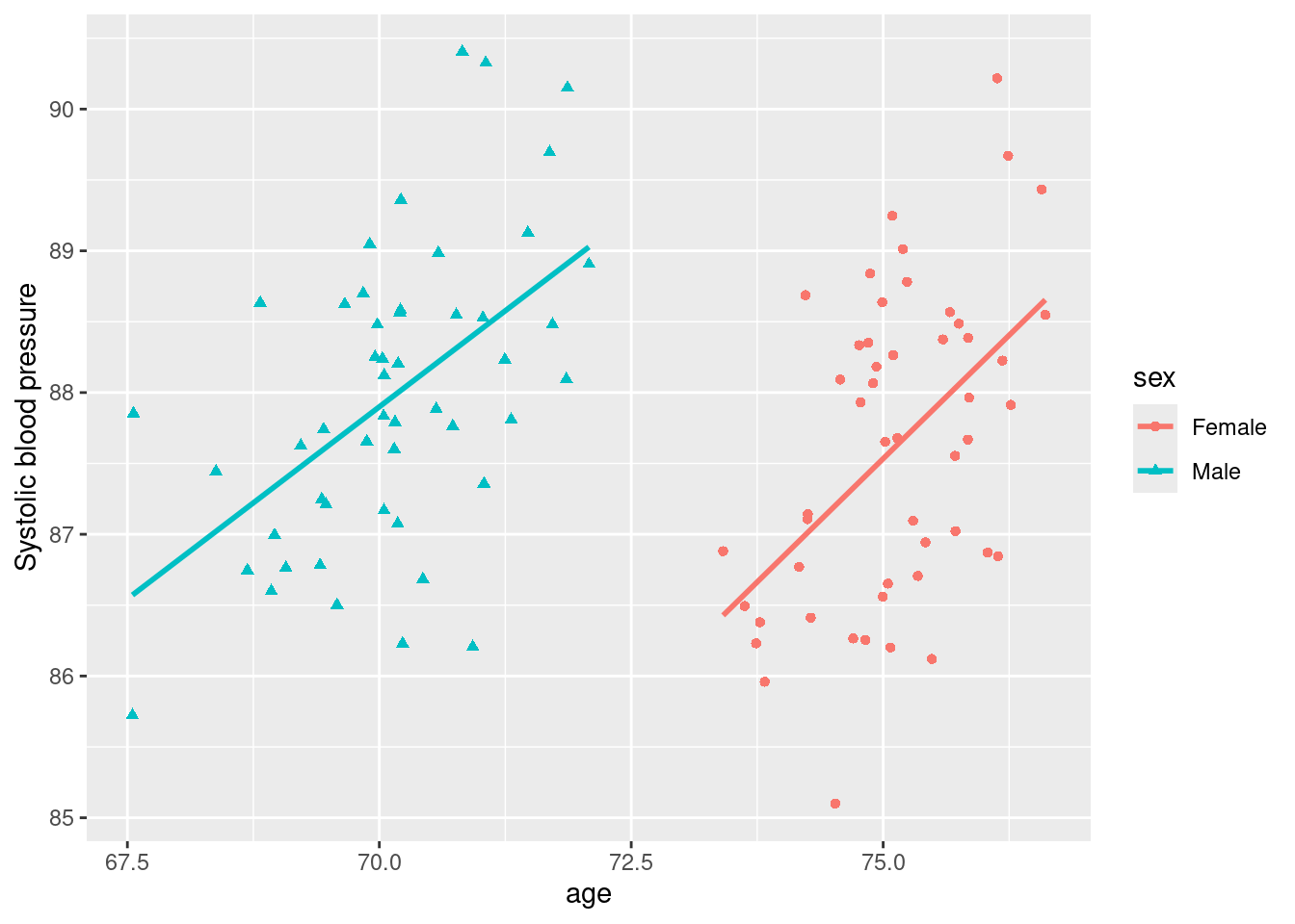
Example 4.1 Consider a study on systolic blood pressure on an elderly population that records the age and sex of each patient. The goal is to determine which of these two covariates are truly associated to blood pressure. In such a simple setting we could do a pretty simple analysis, such as fitting a linear regression model with both covariates and obtaining confidence intervals and P-values. However, for illustration suppose that we use the BIC to choose the best model.
We simulate a dataset that reflects practical difficulties that one may encounter. Suppose that truly both age and gender are associated to blood pressure (as occurs in real life) but that age and gender are correlated in a challenging way. Specifically, suppose that women are older than men by 5 years on average (as occurs in real life, where in developed countries women live roughly 5 years more than mean).
Code
The scatterplot below shows that, if one fits a model with both age and sex, it should be clear that both are associated to blood pressure. However, if one were to ignore sex then blood pressure and age would appear uncorrelated. More precisely, the marginal correlation between blood pressure and age alone is 0.02. Likewise, if one were to ignore age, then it would appear that blood pressure is unrelated to gender (the mean blood pressure is 75.1 for females and 70.1 for males).
Code
Since there are only four models we can easily obtain the BIC for each. We use includevars to force the inclusion of the intercept, i.e. do not consider models that exclude the intercept.
As shown below, the best model according to the BIC includes both age and sex, recovering the data-generating truth.
The second best model however is the intercept-only model, as we expect given that blood pressure has little marginal association to either age or sex alone.
Code
## # A tibble: 4 × 2
##   modelid   bic
##   <chr>   <dbl>
## 1 1,2,3    287.
## 2 1        310.
## 3 1,3      312.
## 4 1,2      315.
In such an example, if one uses a CDA algorithm starting at the intercept-only model then one would not add age nor gender (adding either variable results in a worse value of the objective function) and hence the algorithm would get stuck at a bad local mode. In contrast, if the CDA algorithm were started at the full model then it would get stuck at the model with best BIC, and return the correct solution.
This example may suggest that one should always start the search at the full model including all covariates. Unfortunately, this strategy does not in general guarantee finding the global mode. For example, if the number of covariates \(p\) is large then the MLE under the full model can be very noisy, hence starting the search there can lead to poor local modes. Further, the strategy is not sensible if \(p>n\) and one wants to restrict the search to models with \(\leq n\) variables, as is typically the case. Instead, for \(p>n\) settings it is common to use variable screening methods to identify promising covariates and then one could initialize the model search there. Our example shows that screening variables based on marginal correlations (which would excluce age and sex from further consideration) may lead to bad local modes.
4.3.1 Optimization methods
There has been tremendous progress in optimization methods to solve the L0 problem in linear regression. Bertsimas, King, and Mazumder (2016) proposed a mixed integer programming to solve the problem to exact optimality when the number of variables \(p\) is in the hundreds, and Bertsimas and Van Parys (2020) a cutting plane method that works for \(p\) in the hundreds of thousands. These methods make use of advanced optimization methods and specialized software.
More recently Hazimeh, Mazumder, and Nonet (2023) developed the R package L0Learn, which implements a heuristic optimization algorithm that combines coordinate descent with local combinatorial search. This algorithm runs extremely quickly for \(p\) in the hundreds of thousands, although there is no strict guarantee of global optimality.
We illustrate how these algorithms perform with an example. Both are implemented in R package modelSelection.
bestEBIC_fastuses a coordinate descent algorithm combined with a local combinatorial search. For Gaussian and binary outcomes, it’s a wrapper to functionL0Learn.fitinL0Learnpackage, see its documentation for details.bestEBICuses an MCMC model search, see Section 4.3.2 for a full description. It takes more time thanbestEBIC_fastbut, if we run it for long enough, it’s guaranteed to find the best model eventually.
Example 4.2 We simulate a dataset where \(n=100\), \(p=200\), the covariate values arise from a multivariate Gaussian with zero mean, unit variances and all pairwise correlations equal to 0.5. Out of the \(p=200\) covariates, only the last 4 truly have an effect, with regression coefficients \(\beta_{197}=-2/3\), \(\beta_{198}=1/3\), \(\beta_{199}=2/3\) and \(\beta_{200}=1\).
Code
The heuristic search in bestEBIC_fast and the longer model search in bestEIC return the same solution: a model that includes variables 197, 199 and 200 but not 198 (which was truly active but had a smaller coefficient).
It’s easy to check that this model has better EBIC than the data-generating truth, intuitively the sample size is not large enough to detect this covariate.
These observations that the algorithms likely returned the global mode, or at least a high-quality local mode.
Both algorithms run in a matter of seconds on my Ubuntu laptop, as shown below.
##    user  system elapsed
## 0.570 0.913 0.111## icfit object
##
## Model with best : X197 X199 X200
##
## Use summary(), coef() and predict() to get inference for the top model
## Use coef(object$msfit) and predict(object$msfit) to get BMA estimates and predictions## user system elapsed
## 2.079 0.948 1.592## icfit object
##
## Model with best EBIC : X197 X199 X200
##
## Use summary(), coef() and predict() to get inference for the top model
## Use coef(object$msfit) and predict(object$msfit) to get BMA estimates and predictionsAn important remark is that EBIC is conservative in adding covariates, so it may fail to detect coefficients that are truly non-zero but small.
In this case, variable 198 really has an effect, but it’s not included in the EBIC solution.
To see this issue in a more promounced example, try repeating this exercise but setting the data-generating beta to a smaller value (e.g. divide its entries by 2). Then EBIC will fail to include most truly non-zero coefficients.
4.3.2 MCMC
We now discuss how to use the MCMC methods discussed in Section 3.2 to find the model that optimizes a given \(L_0\) criterion. Let \(C_\gamma= - 2 L_\gamma + \lambda \mbox{dim}(\boldsymbol{\theta}_\gamma)\) be an arbitrary \(L_0\) criterion as defined in (4.1). The main idea is to define a probability distribution on \(\gamma\) as follows \[\begin{align} \pi(\gamma)= \frac{e^{-C_\gamma/2}}{\sum_{\gamma' \in \Gamma} e^{-C_{\gamma'}/2}}. \tag{4.3} \end{align}\] Clearly \(\pi(\gamma) \in [0,1]\) and \(\sum_{\gamma} \pi(\gamma)=1\), defining a probability distribution. It is also to see that if a model \(\boldsymbol{\gamma}^*\) minimizes \(C_\gamma\) then it also maximizes \(\pi(\boldsymbol{\gamma})\).
Therefore, one can use MCMC to sample from \(\pi(\boldsymbol{\gamma})\), and by definition one is more likely to sample \(\boldsymbol{\gamma}^*\) than any other model (upon MCMC convergence, and assuming that \(\boldsymbol{\gamma}^*\) is unique).
One can replace the numerator in (4.3) by any positive function that’s decreasing in \(C_\gamma\) (and adjust the denominator analogously). In particular, the term \(C_\gamma/2\) could be replaced by \(C_\gamma/c\) for any \(c>0\). The motivation for (4.3) is that, when \(C_\gamma\) are the BIC or EBIC, then there is an asymptotic connection between \(\pi(\boldsymbol{\gamma})\) and posterior probabilities obtained from a Bayesian model selection setting. For example, this facilitates transferring theoretical guarantees for MCMC algorithms that were obtained in a Bayesian setting to \(L_0\) criteria (Section 3.2).
4.4 Exercises
Exercise 4.1 Consistency of AIC and BIC. Suppose that we want to compare two nested models \(\boldsymbol{\gamma} \subset \boldsymbol{\gamma}'\), where \(\boldsymbol{\gamma}'\) adds a single parameter to \(\boldsymbol{\gamma}\). Suppose that data are truly generated by \(\boldsymbol{\gamma}\) (the simpler model signifying the null hypothesis), and that the likelihood-ratio statistic \(2(L_{\gamma'} - L_{\gamma}) \stackrel{D}{\longrightarrow} \chi_1^2\) as \(n \to \infty\) (as is the case for regular linear and generalized linear models, for example). Show that as \(n \to \infty\), the probability that the AIC selects \(\boldsymbol{\gamma}\) does not go to 1, whereas for BIC it does go to 1. Discuss how your findings for the AIC compare to a P-value based test that uses a fixed significance level of 0.05.
The AIC chooses model \(\boldsymbol{\gamma}'\) over \(\boldsymbol{\gamma}\) whenever \[\begin{align*} - 2 L_{\gamma'} + 2 \mbox{dim}(\boldsymbol{\theta}_{\gamma'}) < - 2 L_{\gamma} + 2 \mbox{dim}(\boldsymbol{\theta}_{\gamma}) \Longleftrightarrow 2[L_{\gamma'} - L_{\gamma}] > 2. \end{align*}\]
Since \[\begin{align*} \lim_{n \to \infty} P \left( 2[L_{\gamma'} - L_{\gamma}] > 2 \right)= P(\chi_1^2 > 2) = 0.157, \end{align*}\] we have positive probability of wrongly selecting the larger model even as \(n \to \infty\). Note that this probability is non-negligible, and above the usual 0.05 that would be obtained with P-value testing and a fixed 0.05 significance level.
Analogous derivations give that the BIC chooses \(\boldsymbol{\gamma}'\) when \(2 [L_{\gamma'} - L_{\gamma}] > \log n\), and in this case \[\begin{align*} \lim_{n \to \infty} P \left( 2[L_{\gamma'} - L_{\gamma}] > \log n \right)= \lim_{n \to \infty} P(\chi_1^2 > \log n) = 0. \end{align*}\]