1 Quick start

Before properly discussing high-dimensional model selection methods, we show some examples to motivate their utility and to provide a quick start for readers who are already familiar with the basics. The examples also illustrate potential pitfalls that are not always sufficiently appreciated.

We focus on sparse inference methods, mainly Bayesian model selection (BMS) and averaging (BMA), L0 criteria like the BIC or EBIC, L1 (LASSO) and adaptive LASSO. For the illustrations we use R package modelSelection. The main functions for regression-type models are modelSelection and bestBIC (along with companions like bestEBIC, bestAIC and bestIC). modelSelection_eBayes provides an empirical Bayes counterpart to modelSelection.

1.1 Popular methods may fail

We consider a simple setting with \(p=3\) covariates and a moderately large sample size \(n=200\), where popular high-dimensional methods fail to recover the truly active covariates. It may feel underwhelming to start a book on high-dimensional model selection with a \(p=3\) example: the message is that if things can go wrong here, they are bound to get worse for larger \(p\). By understanding what can go wrong in such a manageable example, the hope is that we learn lessons that can be valuable in harder ones, and we better understand what different methods can bring to the table.

Suppose that data are truly generated as follows: \[\begin{align*} x_{i1} & \sim N(0,1) \\ x_{i2} & \sim N(0,1) \\ x_{i3} & \sim N(x_{i1} - x_{i2}, \sigma=0.2) \\ y_i & \sim N(x_{i1} - x_{i2}, \sigma=0.5) \end{align*}\] with independence across \(i=1,\ldots,n\). That is, \(y_i\) truly depends on \(x_{i1}\) and \(x_{i2}\) but not on \(x_{i3}\). The complicating issue is that \(x_{i3}\) is a near-copy of the mean of \(y_i\), and hence the marginal correlation between \(x_{i3}\) and \(y_i\) is high.

Code

library(modelSelection)
library(glmnet)
library(tidyverse)
library(mvtnorm)
set.seed(1234) 
n <- 200
x1 <- rnorm(n)
x2 <- rnorm(n)
x3 <- x1 - x2 + rnorm(n,sd=.2)
x <- cbind(x1, x2, x3)
y <- x1 - x2 + rnorm(n)
df <- data.frame(y, x1, x2, x3)

To show that this is actually an easy exercise, we fit via least-squares the model that includes all covariates. The results correctly suggest that the third covariate could be conceivably dropped, whereas covariates 1-2 are highly statistically significant.

Code

summary(lm(y ~ -1 + ., data=df))

## 
## Call:
## lm(formula = y ~ -1 + ., data = df)
## 
## Residuals:
##      Min       1Q   Median       3Q      Max 
## -2.83454 -0.64344 -0.05624  0.60601  2.49699 
## 
## Coefficients:
##    Estimate Std. Error t value Pr(>|t|)    
## x1  1.13570    0.33100   3.431 0.000732 ***
## x2 -1.05736    0.33124  -3.192 0.001644 ** 
## x3 -0.02529    0.32816  -0.077 0.938637    
## ---
## Signif. codes:  0 '***' 0.001 '**' 0.01 '*' 0.05 '.' 0.1 ' ' 1
## 
## Residual standard error: 0.9501 on 197 degrees of freedom
## Multiple R-squared:  0.705,  Adjusted R-squared:  0.7005 
## F-statistic: 156.9 on 3 and 197 DF,  p-value: < 2.2e-16

The issue is that when the number of covariates \(p\) is large, possibly larger than the sample size \(n\), fitting a model that includes all parameters is often less reliable (the parameter estimates are less precise). High-dimensional methods use other strategies to identify the truly active covariates. A popular strategy is the LASSO (or \(L_1\) regularization) of (Tibshirani 1996), which can quickly obtain parameter estimates for all values of its regularization (or penalty) hyper-parameter. As one increases the penalty, the LASSO solution moves from the model excluding all covariates to first including \(x_{i3}\) (the variable most correlated with \(y_i\)), and subsequently to adding \(x_{i1}\) and \(x_{i2}\), without ever dropping \(x_{i3}\). That is, the data-generating model is not recovered by any value of the penalization parameter.

Code

fit <- glmnet(x=x, y=y, family='gaussian', alpha=1, intercept=FALSE)
models <- unique(t(as.matrix(coef(fit)) != 0))
models

##     (Intercept)    x1    x2    x3
## s0        FALSE FALSE FALSE FALSE
## s1        FALSE FALSE FALSE  TRUE
## s22       FALSE  TRUE FALSE  TRUE
## s34       FALSE  TRUE  TRUE  TRUE

In contrast, the Bayesian information criterion (BIC) of Schwarz (1978) (see Section 4.1), correctly identifies the data-generating model. bestBIC enumerates all \(2^3=8\) models resulting from the inclusion/exclusion of the 3 covariates, and finds the model with best (lowest) BIC. We use the R formula y ~ -1 + . to consider all variables in the data (other than y) as covariates, and set -1 to exclude the intercept, since it’s not needed in this example). We set verbose=FALSE to avoid printing progress information and cluttering the book.

In cases where \(p\) is large, bestBIC uses MCMC to explore the model space. A computationally faster alternative is to use heuristics, for example finding the model with best BIC among those visited in the LASSO or adaptive LASSO path (Zou (2006)), using a coordinate descent algorithm or local combinatorial searches (Hazimeh, Mazumder, and Nonet (2023), R package L0Learn), see Section 4. Function bestBIC_fast in modelSelection implements such heuristics.

Code

fit <- bestBIC(y ~ -1 + ., data=df, verbose=FALSE)
print(fit)

## icfit object
## 
## Model with best  BIC :  x1 x2 
## 
## Use summary(), coef() and predict() to get inference for the top model
## Use coef(object$msfit) and predict(object$msfit) to get BMA estimates and predictions

Fitting the selected model via least-squares shows that both covariates are highly statistically significant.

Code

summary(fit)

## 
## Call:
## glm(formula = f, family = family2glm(ms$family), data = data)
## 
## Coefficients:
##    Estimate Std. Error t value Pr(>|t|)    
## x1  1.11070    0.06605   16.82   <2e-16 ***
## x2 -1.03235    0.06688  -15.44   <2e-16 ***
## ---
## Signif. codes:  0 '***' 0.001 '**' 0.01 '*' 0.05 '.' 0.1 ' ' 1
## 
## (Dispersion parameter for gaussian family taken to be 0.8981151)
## 
##     Null deviance: 602.82  on 200  degrees of freedom
## Residual deviance: 177.83  on 198  degrees of freedom
## AIC: 550.07
## 
## Number of Fisher Scoring iterations: 2

Above we used a single simulated dataset for illustration, but this phenomenon occurs more generally. The table below shows the proportion of times that each covariate was selected among 1,000 simulations, for \(n=200\) and \(n=1000\), when using the BIC, LASSO and adaptive LASSO (penalization parameter chosen by BIC). It also shows results for the fast model search heuristic of Hazimeh, Mazumder, and Nonet (2023) (R package L0Learn). The code to reproduce these results can be unfolded by clicking below.

Click to show code

Code

#Function to simulate one dataset of size n
simdata <- function(n) {
  x1 <- rnorm(n)
  x2 <- rnorm(n)
  x3 <- x1 - x2 + rnorm(n,sd=.2)
  x <- cbind(x1, x2, x3)
  y <- x1 - x2 + rnorm(n)
  df <- data.frame(y, x1, x2, x3)
  return(df)
}

#Function to simulate nsims datasets of size n and obtain
#the proportion of times that each covariate is selected
proportionSelected <- function(nsims, n) {
  sel.L0Learn <- sel.L1 <- sel.adaL1 <- sel.bic <- matrix(NA, nrow=nsims, ncol=3)
  for (i in 1:nsims) {
    df <- simdata(n)
    fit.L0Learn <- bestBIC_fast(y ~ -1 + ., data=df, fastmethod='L0Learn', verbose=FALSE)
    fit.L1 <- bestBIC_fast(y ~ -1 + ., data=df, fastmethod='L1', verbose=FALSE)
    fit.adaL1 <- bestBIC_fast(y ~ -1 + ., data=df, fastmethod='adaptiveL1', verbose=FALSE)
    fit.bic <- bestBIC(y ~ -1 + ., data=df, verbose=FALSE)
    sel.L0Learn[i,] <- fit.L0Learn$varnames %in% fit.L0Learn$topmodel  
    sel.L1[i,] <- fit.L1$varnames %in% fit.L1$topmodel  
    sel.adaL1[i,] <- fit.adaL1$varnames %in% fit.adaL1$topmodel  
    sel.bic[i,] <- fit.bic$varnames %in% fit.bic$topmodel  
  }
  nn <- c('BIC', 'LASSO BIC', 'ALASSO BIC', 'L0Learn')
  propsel <- rbind(colMeans(sel.bic), colMeans(sel.L1), colMeans(sel.adaL1), colMeans(sel.L0Learn))
  propsel <- data.frame(Method=nn, propsel)
  return(propsel)
}

propsel.n200 <- proportionSelected(nsims=1000, n=200)
propsel.n1000 <- proportionSelected(nsims=1000, n=1000)
propsel.n200$n <- 200
propsel.n1000$n <- 1000

propsel <- rbind(propsel.n200, propsel.n1000)
write.table(propsel, "tables/lassofailure.txt", row.names=FALSE, col.names=TRUE, sep="\t")

	n = 200			n = 1,000
Method	X1	X2	X3	X1	X2	X3
BIC	0.721	0.722	0.291	0.994	0.994	0.006
LASSO BIC	0.491	0.489	0.547	0.993	0.993	0.637
ALASSO BIC	0.491	0.489	0.531	0.993	0.993	0.007
L0Learn	0.530	0.528	0.497	0.993	0.993	0.522

BIC is the best method, including the truly active covariates 1-2 and excluding the truly inactive covariate 3 more frequently than the other methods. LASSO-BIC and L0Learn wrongly include the third covariate in 50% of the simulations or more, that is they incur a very high false positive rate, and the situation does not improve as \(n\) grows. Interestingly, adaptive LASSO performs similarly to LASSO for \(n=200\) and similarly to BIC for \(n=1,000\).

Remark: LASSO-BIC uses BIC to select the best model, so how can its results be so different from BIC? The reason is that LASSO-BIC only evaluates the BIC for models visited by the LASSO path, and the latter may not include the data-generating model. Similar issues are encountered when setting the LASSO penalty with cross-validation (results not shown).

These findings are not a coincidence. There is theory for LASSO explaining that it can be expected to select a super-set of the truly active variables (the so-called screening property), but that this may contain false positives when the covariates are correlated in challenging ways (more precisely, when the so-called irrepresantability condition is not met, see Section 4.2). The adaptive LASSO consistently identifies the truly active covariates under less stringent conditions than LASSO, as illustrated in our findings for \(n=1,000\). Alas, in this example, when \(n=200\) its performance leaves much to be desired.

In contrast, L0 criteria like the BIC have better theoretical properties in such settings, and the same holds for Bayesian model selection methods. Admittedly computation is harder, but given the potential improvements in variable selection we argue that one should at least try. As we shall see, finding a (possibly approximate) solution is often feasible. Following Tukey’s motto, we argue that an approximate solution to the right problem is preferable to an exact solution to the wrong problem.

1.2 Model uncertainty

A limitation of L0 criteria is that they ignore the uncertainty in the selected model, i.e. we’re not completely sure that it’s the correct one. Bayesian model selection (BMS) is a strategy to portray model choice uncertainty, and we discuss it in some detail in Chapter 2. BMS requires setting a prior distribution on the models and on the parameters for each model. For now, we illustrate the use of BMS by setting default priors (Beta-Binomial prior on the models, product MOM prior with default prior precision on the coefficients).

Code

priorCoef <- momprior()
priorModel <- modelbbprior()
fit.bms <- modelSelection(y ~ -1 + ., data=df,
                     priorCoef=priorCoef, priorModel=priorModel,
                     verbose=FALSE)

BMS provides posterior model probabilities, a Bayesian measure of the certainty that each model is the correct one. Below we show the five models with highest posterior probability. Only two models have a non-negligible posterior probability. The top model includes covariates 1-2 (the data-generating trugh) and has posterior probability 0.64, whereas the second model includes all 3 covariates and has posterior probability 0.34. Given that covariate 3 is a near-copy of the outcome, and that we have a limited amount of data (\(n=200\)), it seems reasonable that we are not completely sure about which of these two models is the correct one.

Code

postProb(fit.bms)[1:5,]

##   modelid family           pp
## 7     1,2 normal 0.6438458284
## 8   1,2,3 normal 0.3442356139
## 2       3 normal 0.0114396003
## 6     1,3 normal 0.0004294816
## 4     2,3 normal 0.0000494759

coef gives Bayesian model averaging (BMA) point estimates, 0.95 posterior intervals, and marginal posterior inclusion probabilities \(P(\theta_j \neq 0 \mid y)\). Below, phi refers to the error variance \(\sigma^2\) (which is included with probability 1). In our example, BMS selects the right covariates and assigns high posterior probability to that solution, as one would ideally wish.

Code

coef(fit.bms)

##              estimate       2.5%      97.5%    margpp
## intercept -0.03478042 -0.0496490 -0.0186861 1.0000000
## x1         0.98915072  0.4862229  1.2980217 0.9885109
## x2        -0.91515357 -1.2267667 -0.4173619 0.9881309
## x3         0.11173227 -0.2092983  0.6156765 0.3561542
## phi        0.90923160  0.7483423  1.1059294 1.0000000

Finally, we can use predict to obtain point predictions and 0.95 posterior predictive intervals.

Code

ypred <- predict(fit.bms)
head(ypred)

##         mean        2.5%      97.5%
## 1 -1.8887400 -2.10166202 -1.6974587
## 2 -0.4435298 -0.53110644 -0.3563479
## 3  0.9606666  0.81105334  1.1089939
## 4 -3.3575365 -3.69164069 -3.0255310
## 5  0.1268887  0.04994996  0.2085443
## 6 -0.2545186 -0.36481107 -0.1450838

1.3 Are computations always hard?

A common objection to Bayesian model selection and \(L_0\) criteria is that they’re computationally unfeasible as the number of covariates \(p\) grows. It is true that the problem is worst-case NP-hard even in canonical linear regression (see for example Natarajan (1995), Cover and Van Campenhout (2007), Foster, Karloff, and Thaler (2015)), in the sense that one can always design a dataset such that finding the best model according to these criteria has an exponential cost in \(p\). However this is in a worst-case scenario, in practice one may be able to solve the problem quickly. In particular as \(n\) grows and under so-called sparsity constraints, \(L_0\) criteria and Bayesian posterior probabilities concentrate on a small subset of models with high probability, which often facilitates model search. These issues are discussed in Chapters 3 and 4, and Chapter 5 discusses important implementation details and further nuances (for example, larger \(n\) makes model-specific calculations harder). For now we provide an example where \(p=200\) and \(n=200\). The first six covariates have non-zero effects \(\beta_1=0.5\), \(\beta_2=0.6\), …, \(\beta_{6}=1\), whereas \(\beta_7=\ldots = \beta_p=0\). The covariates are generated from a multivariate Gaussian with unit variances and 0.7 pairwise correlations, which is a moderately strong correlation structure.

Code

n <- p <- 200
sigma <- diag(p)
sigma[upper.tri(sigma)] = sigma[lower.tri(sigma)] = 0.7
x <- rmvnorm(n, sigma=sigma)
beta <- matrix(c(seq(0.5,1,by=0.1), rep(0,p-6)), ncol=1)
y <- rnorm(n, x %*% beta)
df <- data.frame(y=y, x)

Given that \(p\) is large here we use the EBIC (Chen and Chen (2008)), an extension of the BIC that’s better suited for high-dimensional problems. As shown below, optimization heuristics return an answer in less than 0.5 seconds in my Ubuntu laptop. The selected model selects all the truly active covariates 1-6 and also covariate 104, which is a false positive. This is a fairly good answer.

Code

system.time(fit.ebicfast <- bestEBIC_fast(y ~ ., data=df, verbose=FALSE))['elapsed']

## elapsed 
##   0.356

Code

fit.ebicfast

## icfit object
## 
## Model with best  :  X1 X2 X3 X4 X5 X6 X104 
## 
## Use summary(), coef() and predict() to get inference for the top model
## Use coef(object$msfit) and predict(object$msfit) to get BMA estimates and predictions

For comparison, the model with best EBIC within the LASSO path misses truly active covariates 1-2, and includes two false positives (covariates 62 and 68).

Code

bestEBIC_fast(y ~ ., data=df, fastmethod='L1', verbose=FALSE)

## icfit object
## 
## Model with best  EBIC :  X3 X4 X5 X6 X62 X68 
## 
## Use summary(), coef() and predict() to get inference for the top model
## Use coef(object$msfit) and predict(object$msfit) to get BMA estimates and predictions

Bayesian model selection via MCMC took longer to run, but still below 3 seconds. The highest posterior probability model matches that selected by the EBIC. We also see that its posterior probability is small, that is there isn’t strong Bayesian evidence that this is the correct model. This seems reasonable, given that \(p\) is large and that covariates are strongly correlated.

Code

system.time(ms <- modelSelection(y ~ -1 + ., data=df, verbose=FALSE))['elapsed']

## elapsed 
##   2.819

Code

head(postProb(ms))

##              modelid family         pp
## 1    1,2,3,4,5,6,104 normal 0.05810229
## 2  2,3,4,5,6,104,199 normal 0.03788968
## 3  2,3,4,5,6,160,199 normal 0.03515450
## 4      2,3,4,5,6,104 normal 0.02808176
## 5 3,4,5,6,40,160,199 normal 0.02629312
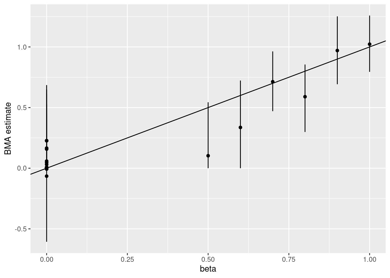
## 6     3,4,5,6,40,199 normal 0.02219088

BMA returns point estimates and 0.95 posterior probability intervals, plotted below. The posterior interval of each \(\beta_j\) contains the data-generating \(\beta_j\) in this example, and the point estimates for the truly zero \(\beta_j\)’s are quite close to zero.

Click to show code

Code

b <- coef(ms)
sel <- !(rownames(b) %in% c('intercept','phi'))
b <- data.frame(b[sel,]) |>
  transform(Covariate = 1:p, beta=beta) |>
  rename(cilow=X2.5., ciup=X97.5.)

myplot <- ggplot(b, aes(x=beta, y=estimate)) +
  geom_point() +
  geom_segment(aes(x=beta, y=cilow, yend=ciup)) +
  labs(y='BMA estimate') +
  geom_abline(slope=1)

Code

myplot

1.4 An Achilles heel

Before we get too excited, let’s illustrate the Achilles heel of standard high-dimensional model selection methods: sparsity and betamin assumptions. The philosophy of these methods is to be conservative in terms of adding parameters, that is avoid using unnecessarily complex models. Intuitively, this strategy seems reasonable when:

Truly most parameters are zero (a sparsity assumption). By being conservative, one avoids false positives (type I errors, in statistical jargon), and since most parameters are zero this is a primary concern.
The truly non-zero parameters are large enough (a betamin assumption), or alternatively the sample size \(n\) is large enough.

If these two assumptions are not met, taking a conservative approach may result in low statistical power to detect parameters that are truly non-zero but small. We discuss these issues and some empirical Bayes strategies to ameliorate them in Chapter 7.

For now, we repeat the previous example but now the non-zero \(\beta_j\)’s are divided by three. Below we report results averaged across 200 independent simulations, both for the larger and the smaller \(\beta\) settings.

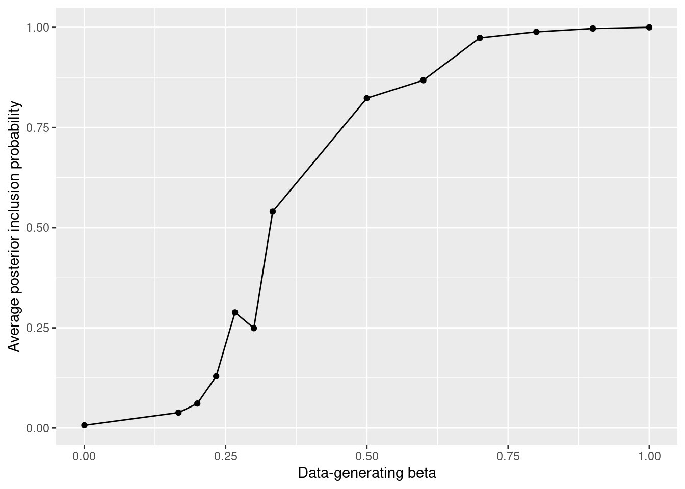
The left panel in the figure below shows that for small \(\beta_j\) there is low statistical power, that is a probability of selecting the corresponding covariates, and that this is an issue for EBIC, LASSO-EBIC and BMA. For BMA this is particularly problematic: the Bayesian uncertainty quantification is off, from a frequentist standpoint. Small \(\beta_j\)’s are assigned a high \(P(\beta_j = 0 \mid y)\), and taking the latter posterior probability at face value would give strong Bayesian evidence that the corresponding covariates have no effect. This example illustrates that BMA results should be interpreted as a conservative analysis where small evidence for inclusion may simply be due to low statistical power, rather than conclusive evidence that the effects are zero.

Click to show code

Code

runsims <- function(n, beta, nsims) {
  varnames <- paste("X", 1:ncol(pp), sep="")
  pp <- matrix(0, nrow=nsims, ncol=length(beta))
  colnames(pp) <- varnames
  sel.ebicfast <- sel.lassoebic <- sel.ms <- pp 
  for (i in 1:nsims) {
    y <- rnorm(n, x %*% beta)
    df <- data.frame(y=y, x)
    # EBIC (fast heuristics)
    top.ebicfast <- bestEBIC_fast(y ~ ., data=df, verbose=FALSE)$topmodel
    sel.ebicfast[i, ] <- varnames %in% top.ebicfast
    # LASSO EBIC
    top.lassoebic <- bestEBIC_fast(y ~ ., data=df, fastmethod='L1', verbose=FALSE)$topmodel
    sel.lassoebic[i, ] <- varnames %in% top.lassoebic
    # BMS
    ms <- modelSelection(y ~ -1 + ., data=df, niter=1000, verbose=FALSE)
    sel.ms[i, which(ms$postMode == 1)] <- TRUE 
    margpp <- coef(ms)[,'margpp']
    pp[i,] <- margpp[-c(1,length(margpp))]
  }
  ans <- data.frame(n = n,
                    variable = 1:length(beta),
                    beta = beta,
                    ebic= colMeans(sel.ebicfast),
                    lasso_ebic = colMeans(sel.lassoebic),
                    bms = colMeans(sel.ms),
                    pp= colMeans(pp))
  return(ans)
}

Code

sim1 <- runsims(n=n, beta=beta, nsims=200)
sim1$simulation <- "Large beta"
sim2 <- runsims(n=n, beta=beta/3, nsims=200)
sim2$simulation <- "Small beta"

simall <- rbind(sim1, sim2) |>
  group_by(simulation, beta, n) |>
  summarize(ebic=mean(ebic), lasso_ebic=mean(lasso_ebic), bms=mean(bms), pp=mean(pp))

write.table(simall, "tables/achilles_quick.txt", row.names=FALSE, col.names=TRUE, sep="\t")

Code

simall <- read.table("tables/achilles_quick.txt", header=TRUE, sep="\t") |>
  group_by(beta) |>
  summarize(ebic=mean(ebic), lasso_ebic=mean(lasso_ebic), bms=mean(bms), pp=mean(pp))

plot1 <- ggplot(simall, aes(x=beta)) +
  geom_line(aes(y=ebic, color='EBIC')) +
  geom_line(aes(y=lasso_ebic, color='LASSO-EBIC')) +
  geom_line(aes(y=bms, color='BMS')) +
  scale_color_manual(
    name = "Method",
    values = c("EBIC" = "black", "LASSO-EBIC" = "red", "BMS" = "blue")
  ) +
  labs(y= 'Proportion of simulations in which variable was selected', x='Data-generating beta')

Code

plot2 <- ggplot(simall, aes(x=beta, y=pp)) +
  geom_line() +
  geom_point() +
  labs(y= 'Average posterior inclusion probability', x='Data-generating beta')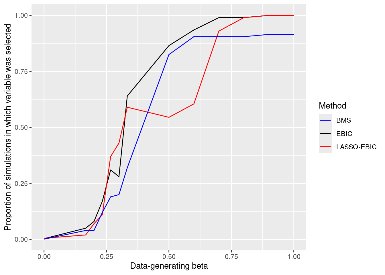

1.5 Beyond linear models

The ideas discussed so far extend well beyond linear and generalized liner models in a relatively seamless manner. For example, one may wish to learn whether covariates have a linear or non-linear effect, or no effect at all, which we discuss in Chapter 6. Another example is learning sparse covariance models such as graphical or factor models, which we discuss in Chapter 9). More advanced uses include learning what covariates to include in a deep learning model, or whether non-linear or high-level interactions are needed.

For now we provide a brief illustration of generalize additive models (GAMs), a popular semi-parametric model to capture non-linear covariate effects. For Gaussian outcomes, the canonical GAM assumes that \[ y_i = \beta_0 + \sum_{j=1}^p \beta_j x_{ij} + \sum_{j=1}^p f_j(x_{ij}) + \epsilon_i \] where \(\epsilon_i \sim N(0,\sigma^2)\) and the \(f_j\)’s must satisfy certain add-to-zero constraints for the model to be identifiable. The interpretation is that \(f_j\) captures deviations from linearity. Note that one could define \(\tilde{f}_j(x_{ij})= \beta_j x_{ij} + f_j(x_{ij})\) and estimate \(\tilde{f}_j\) directly, but then testing whether \(\tilde{f}_j(z)=0\) for all \(z\) just tells us whether covariate \(j\) has a effect, rather than whether it is linear or non-linear. A popular strategy to parameterize \(f_j\) is via B-spline functions, and that’s what we use here.

We simulate a dataset with 10 covariates where the first six have a linear effect, the seventh a non-linear effect and the remaining 3 have no effect on the outcome.

Code

n <- 200; p <- 10
beta <- matrix(c(seq(0.5,1,by=0.1), rep(0,p-6)), ncol=1)
sigma <- diag(p)
sigma[upper.tri(sigma)] <- sigma[lower.tri(sigma)] <- 0.5
x <- rmvnorm(n, sigma=sigma)
mu <- x %*% beta + cos(pi * x[,7])
y <- rnorm(n, mu, sd=1)
df <- data.frame(y=y, x)

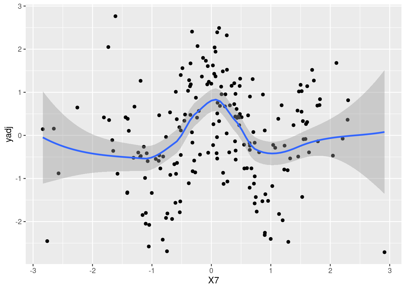
While this is not a very hard exercise, it’s also not completely trivial. For example, a scatter-plot of the outcome versus the seventh covariate (left panel below) doesn’t suggest that it may have a non-linear effect. If instead one plots partial residuals obtained after removing the effect of covariates 1-6, that is \(e_i= y_i - \sum_{j=1}^6 x_{ij} \beta_j\), the non-linear effect becomes apparent (right panel). That is, in this example the key to discover the non-linear association is to adequately capture the effect of other covariates.

Click to show code

Code

df2plot <- data.frame(y, x) |>
  transform(yadj = y - x %*% beta, muadj = cos(pi * X7))

p1 <- ggplot(df2plot, aes(x=X7, y=y)) +
  geom_point() +
  geom_smooth()

p2 <- ggplot(df2plot, aes(x=X7, y=yadj)) +
  geom_point() +
  geom_smooth()

## `geom_smooth()` using method = 'loess' and formula = 'y ~ x'
## `geom_smooth()` using method = 'loess' and formula = 'y ~ x'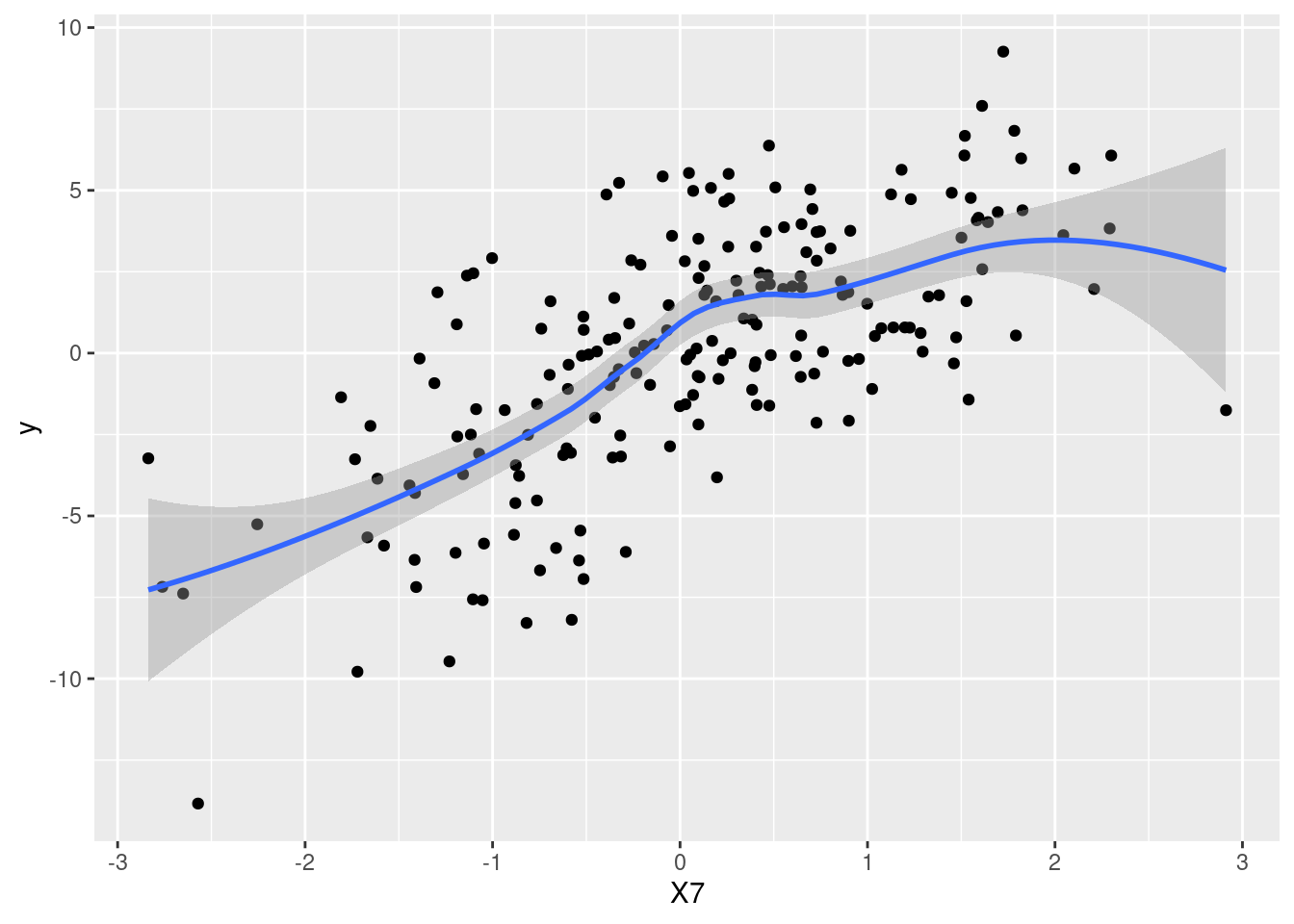

Let us perform Bayesian model selection on these data. The table below displays the marginal posterior probability that each covariate has a linear and a non-linear effect. Covariates 1-6 are correctly flagged as only having a linear effect, covariate 7 as having a non-linear effect, and for covariates 8-10 there is no strong evidence for either a linear or non-linear effect.

Code

fit.gam <- modelSelection(y ~ ., data=df,
                     smooth = ~ X1 + X2 + X3 + X4 + X5 + X6 + X7 + X8 + X9 + X10,
                     priorCoef=priorCoef,
                     priorModel=priorModel, verbose=FALSE)
b <- coef(fit.gam)

Click to show code

Code

pp <- data.frame(id= rownames(b), margpp=b[,'margpp']) |>
  dplyr::filter(id != "(Intercept)", id != "phi") |>
  transform(idshort = gsub("\\.s[0-9]+", "\\s", id)) |>
  dplyr::select(idshort, margpp) |>
  unique() |>
  transform(idshort= gsub("s", " non-linear", idshort))

pp.lin <- dplyr::filter(pp, !grepl("non-linear", idshort))
pp.nonlin <- dplyr::filter(pp, grepl("non-linear", idshort))
pp <- data.frame(variable= rownames(pp.lin), linear=pp.lin[,"margpp"], nonlinear= pp.nonlin[,"margpp"])

variable	linear	nonlinear
X1	0.9999716	0.0001443
X2	1.0000000	0.0000374
X3	1.0000000	0.0004667
X4	1.0000000	0.0001289
X5	1.0000000	0.0014218
X6	1.0000000	0.0003170
X7	1.0000000	1.0000000
X8	0.1905414	0.0000257
X9	0.0780882	0.0000183
X10	0.0173677	0.0000105

References

Chen, J., and Z. Chen. 2008. “Extended Bayesian Information Criteria for Model Selection with Large Model Spaces.” Biometrika 95 (3): 759–71.

Cover, Thomas M, and Jan M Van Campenhout. 2007. “On the Possible Orderings in the Measurement Selection Problem.” IEEE Transactions on Systems, Man, and Cybernetics 7 (9): 657–61.

Foster, D., H. Karloff, and J. Thaler. 2015. “Variable Selection Is Hard.” In Conference on Learning Theory, 696–709.

Hazimeh, Hussein, Rahul Mazumder, and Tim Nonet. 2023. “L0learn: A Scalable Package for Sparse Learning Using L0 Regularization.” Journal of Machine Learning Research 24 (205): 1–8.

Natarajan, B. K. 1995. “Sparse Approximate Solutions to Linear Systems.” SIAM Journal on Computing 24 (2): 227–34.

Schwarz, G. 1978. “Estimating the Dimension of a Model.” The Annals of Statistics 6: 461–64.

Tibshirani, R. 1996. “Regression Shrinkage and Selection via the Lasso.” Journal of the Royal Statistical Society, B 58: 267–88.

Zou, H. 2006. “The Adaptive LASSO and Its Oracle Properties.” Journal of the American Statistical Association 101 (476): 1418–29.